Postgres

Core Architecture

Process Model (Postmaster, Backends, Background Workers)

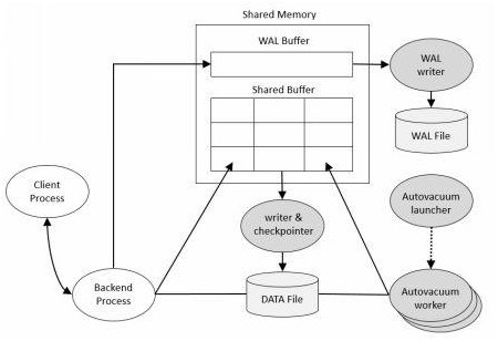
PostgreSQL uses a multi-process architecture for stability and isolation. The Postmaster (also called the postgres daemon) is the parent process that starts when the database server is launched. The Postmaster initializes shared memory and launches essential background processes on startup. It listens for client connection requests; when a new client connects, the Postmaster forks a new backend process& dedicated to that session. In other words, each database connection is handled by its own client backend process, providing isolation (a crash in one backend does not crash others) at the cost of some overhead. All these processes are visible in the OS process table (on Unix systems, the postgres processes form a tree under the Postmaster). severalnines.com

Each backend process executes queries on behalf of its client and communicates results back. The number of concurrent backends is limited by the max_connections setting (default around 100). Backends are stateful and maintain session-specific context and local memory (for sorting, hashing, etc., discussed in the Memory section). When the client disconnects, its backend process exits, freeing resources.

Beyond backends, PostgreSQL runs a suite of background worker processes to handle various maintenance and I/O tasks. Important background processes include:

• Logger – writes server logs to disk (capturing errors, messages).
• Checkpointer – periodically takes a checkpoint by flushing dirty shared buffers (modified data pages) to disk. This reduces recovery time by ensuring a point from which the database can start applying WAL (Write-Ahead Log) during crash recovery.
• Background Writer (writer) – continuously writes some dirty pages to disk in the background to spread out I/O load.
• WAL Writer – flushes the WAL buffer to the WAL files on disk regularly (and at transaction commit), ensuring WAL data is durably stored.
• Autovacuum Launcher – manages autovacuum workers which reclaim space by vacuuming tables and indexes and prevent transaction ID wraparound issues. The launcher wakes up periodically and forks worker processes to clean tables with too many dead tuples.
• Archiver – if WAL archiving is enabled, this process copies completed WAL segment files to an archive location (e.g. for backups).
• Statistics Collector – (for PostgreSQL versions before 15) collects runtime statistics (table usage, index usage, etc.) and writes them to stats files. Note: PostgreSQL 15 removed the separate stats collector process, replacing it with a shared memory statistics system postgresql.org.

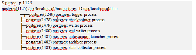
These background processes are all forked by the Postmaster at startup (except autovacuum workers, which are forked on demand by the autovacuum launcher). The Postmaster is thus the root of all other postgres processes. This model (one process per connection + helper processes) is different from a threaded model – it trades higher per-connection overhead for strong memory isolation and resilience.

Example: If 10 clients connect to the database, the Postmaster will spawn 10 backend processes (each handling one client), and the standard background processes will be running to handle logging, checkpointing, WAL writing, etc. If one backend crashes, it does not directly corrupt other sessions – the Postmaster will detect the crash and can terminate or restart the system gracefully as needed. The following diagram illustrates PostgreSQL’s process model with the Postmaster, two client connections (with their backends), and some background workers:

Memory Architecture (Shared Buffers, WAL Buffers, work_mem, maintenance_work_mem)

PostgreSQL’s memory is divided into shared memory (global to all processes) and per-process memory. Shared memory is allocated at server start and is accessible by all backend and background processes. It contains crucial global data structures for caching and synchronization. The two largest components of shared memory are the Shared Buffer pool and the WAL Buffer: dbsguru.com

• Shared Buffers: This is the main RAM cache for database pages (disk blocks). Whenever data pages are read from disk or written, they pass through the shared buffer cache. Frequently accessed pages stay in memory to minimize disk I/O. Shared buffers are managed with an LRU-replacement strategy (with adjustments to prioritize “hot” pages) and use a partitioned locking mechanism to allow concurrent access with minimal contention. The goal is to keep frequently used blocks in memory as long as possible, reducing costly disk reads. If a page is modified in shared buffers, it’s marked “dirty” but not immediately written to disk – the background writer or checkpointer will flush it later. The size of the shared buffer pool is controlled by the shared_buffers parameter (e.g. if set to 128MB, about 16,384 8KB pages can be cached).
• WAL Buffers: The WAL (Write-Ahead Log) buffer is a small amount of shared memory used to temporarily store WAL records (log entries describing database changes) before they are written to the WAL files on disk. By default this buffer is modest (often a few hundred kilobytes, e.g. 16 WAL pages) since WAL is flushed frequently. The WAL buffer allows transactions to group multiple changes in memory and write them to disk sequentially, improving throughput. The WAL records in this buffer contain metadata sufficient to reconstruct data changes during recovery. The contents of WAL buffers are written out to disk on each transaction commit (or sooner if the buffer fills or after a timeout) by the WAL writer process.

Shared memory also includes other structures: lock tables and latch mechanisms for synchronization, the commit log (pg_xact) and clog buffers that track transaction commit status, and the shared catalog cache, among others. However, the shared buffer cache and WAL buffer are the largest and most performance-critical shared memory areas.

Each backend also has its own private memory for query execution. Key per-backend memory settings include:

• work_mem: This parameter defines the memory available for internal sort operations and hash tables within a query (per sort or hash operation). For example, when a query needs to sort rows (ORDER BY, aggregates, etc.) or build a hash table for a hash join, it will use up to work_mem bytes before spilling to disk (using temp files). By default this might be 4MB, meaning each sort or hash can use 4MB of RAM. Note that a single complex query might perform multiple sorts or hashes in parallel, each getting its own work_mem allowance. Tuning work_mem is important: too low and queries will spill to disk (slowing down), too high and many concurrent queries could exhaust memory. Example: If work_mem = 4MB and a query does a large ORDER BY on a table, it can sort up to 4MB of data in memory; if the dataset is larger, PostgreSQL will write the overflow to a temporary file on disk.
• maintenance_work_mem: This is a larger memory area used for maintenance operations like VACUUM, CREATE INDEX, ALTER TABLE ADD FOREIGN KEY, and other operations that might need to sort or process large amounts of data for maintenance tasks. The default is higher (e.g. 64MB) to allow vacuum and index builds to complete faster. Each running maintenance task (manual VACUUM, autovacuum worker, index creation, etc.) can use up to this amount of memory. For autovacuum, there is also a parameter autovacuum_work_mem (which if set to -1 means it defaults to maintenance_work_mem). For instance, if maintenance_work_mem = 128MB, an index creation can use up to 128MB RAM for sorting index entries, which significantly speeds up index building compared to using the smaller work_mem limit.
• temp_buffers: Each backend has a allocation for temporary table data if the session creates temporary tables. This is controlled by temp_buffers (default 8MB). These buffers are allocated per session for handling access to temp tables (which are session-local). Memory Architecture: The diagram below shows the separation between shared memory (accessible to all processes) and each process’s local memory:

Storage Architecture (Heap Files, Pages, Tuples, TOAST, Large Objects)

PostgreSQL stores database data on disk in a cluster of files in the data directory (commonly referred to as PGDATA). The data is organized by database and tablespace, but at the lowest level, each table or index is stored in one or more files on disk. A table (heap) is stored in a file identified by a numeric identifier (the table’s filenode, often matching its OID). Each such file is a sequence of fixed-size pages (usually 8KB each by default). Pages are sometimes called disk blocks. PostgreSQL does not allow a single row to span multiple pages (except via TOAST, discussed below), so the page size is a hard upper limit on row size without TOAST. docs.hevodata.com

If a table grows larger than 1GB, PostgreSQL automatically divides it into multiple segment files (each up to 1GB, with file names like oid.1, oid.2, etc.) docs.hevodata.com. This is transparent to the user and done to accommodate large tables on filesystems with file size limits.

Page Structure: Each 8KB page contains a page header (with metadata like LSN – the log sequence number of the last WAL record affecting the page, checksum, free space pointers, etc.), an array of item pointers (line pointers) that serve as offsets to the actual row data, the row tuples (item contents) themselves, and some free space in between for future row growth or new insertions. When new rows are inserted or updated, PostgreSQL fills the free space on pages; when rows are deleted or updated (leaving dead tuples), the space becomes available for reuse (tracked in free space maps). A page can hold multiple tuples (the exact number depends on row size). If a row is too large to fit on a page, PostgreSQL will off-load its large field values using TOAST (explained shortly).

Heap Tuples (Rows): A tuple is a single row version stored on a page. Each tuple has its own tuple header (storing metadata such as its length, a pointer to its OID or presence in indexes, and crucially the MVCC timestamps: the xmin and xmax transaction IDs – identifying which transaction inserted it and which transaction (if any) deleted it). The tuple header also contains flags for null values, etc. Following the header, the tuple stores the actual row columns. Example: If you insert a row into a table, PostgreSQL will find a page with enough free space (using the free space map) and place the tuple there, setting its xmin to the inserting transaction’s ID. If you later update that row, PostgreSQL will create a new tuple (version) on potentially the same or another page (if not enough space), set its xmin to the updating transaction, and mark the old tuple’s xmax to the updating transaction ID (to denote it as outdated) – thus preserving the old version for MVCC. This means multiple versions of a row can reside in the heap, and the visibility rules (MVCC) determine which version is seen by a transaction (see Transaction Management section).

Table Files and Auxiliary Files: For each table, PostgreSQL maintains not only the main data file but also two auxiliary files: a Free Space Map (FSM) and a Visibility Map (VM). The FSM (stored in a file with suffix _fsm) records how much free space exists in each page of the table, so the server can quickly find a page with space for a new row. The Visibility Map (file with suffix _vm) stores flags for each page indicating whether all tuples on that page are visible to all transactions (a page with no recent modifications). The visibility map helps optimize vacuuming and index-only scans – for example, an index-only scan can skip reading heap pages if the VM indicates all tuples on that page are visible (no need to check heap for recent changes). Each table’s FSM and VM are updated as inserts, updates, and vacuuming occur. (Indexes have an FSM but no VM, since visibility pertains to heap data only.)

Disk Layout Example: Consider a table accounts(id INT, balance NUMERIC) with 1000 rows. Those rows might occupy, say, 20 pages of 8KB each (50 rows per page). The table will have one main file (or multiple segments if large), plus accounts_fsm and accounts_vm. If you delete 100 rows, those rows’ tuples remain in the pages as dead tuples until vacuum removes them, but the free space map will record extra free space on those pages. An index on id would be stored separately in its own file (B-tree structure) and have its own FSM file.

TOAST (Oversized Attribute Storage): Because table pages are fixed-size, very large field values (such as large text or BLOBs) cannot fit in-line if they exceed the page size. To handle this, PostgreSQL uses TOAST (The Oversized-Attribute Storage Technique) for automating storage of large values off-page. When a row contains a value that exceeds a threshold (by default around 2KB for a field), PostgreSQL will compress the value (if possible) and store it in a separate TOAST table, which is an implicit auxiliary table for the main table. The original table’s tuple will keep only a pointer (a TOAST pointer datum) in that field, instead of the full large value. The TOAST pointer includes information to locate the external data (like the OID of the toast table and chunk IDs). postgresql.org

A TOAST table stores large values in chunks (typically ~2KB chunks). Each chunk is a row in the toast table, with an ID linking it to the original value and a sequence number. By default, PostgreSQL tries to compress the field and break it into chunks such that 4 chunks fit in one page (around 2KB each). For example, if you have a 1MB bytea (binary data) value in a column, the main table will store a small pointer, and the TOAST table will contain about 500 chunks of ~2KB each to represent that 1MB value. The whole process is transparent to the user: when you SELECT the large column, PostgreSQL will detoast it (retrieve all chunks and recombine/decompress them) automatically. TOAST makes handling of large values seamless up to PostgreSQL’s limit of 1GB per field (imposed by the pointer format). Most built-in large types (text, varchar, bytea, etc.) are TOAST-able. cloudthat.com

Large Objects: In addition to TOAST, PostgreSQL provides a Large Object (LOB) facility for storing very large values in a special way (using pg_largeobject system table). This is an older interface where large objects are treated with an ID and read/write in chunks via special functions or drivers. Internally, the large object data is also chunked in 2KB segments similar to TOAST. Many applications today simply use bytea (which leverages TOAST) for storing big binary data, but the LOB facility is still available (useful for streaming large files in/out).

Storage & TOAST: The following diagram illustrates how a table’s data is organized into pages and how a large field value is stored out-of-line via TOAST:

Note: Because PostgreSQL MVCC retains old tuple versions, tables can experience bloat (accumulation of dead tuples). Regular VACUUM operations are needed to reclaim space by removing dead tuples and updating the FSM/VM. Also, as transactions commit, the visibility map is updated (marking pages all-visible when appropriate), enabling index-only scans and optimizing future vacuums.

Write-Ahead Logging (WAL) – Durability and Recovery

PostgreSQL employs Write-Ahead Logging (WAL) to guarantee durability and crash recovery. The central idea of WAL is simple but powerful: before any change is applied to data files (tables or indexes), an undo/redo record of that change is first written to the WAL log and flushed to stable storage. Only after the WAL record is securely on disk can the in-memory change be written to the table on disk (usually deferred). This ensures that if the database crashes, it can recover by “replaying” the log of changes and not lose any committed transactions. WAL thus provides the “D” (Durability) in ACID. postgresql.org

The WAL in PostgreSQL is a sequence of binary log files (16MB each by default) recording every data modification (insert, update, delete, DDL changes, etc.). Each WAL record describes a change at the disk page level or a logical level that can be redone. WAL records are identified by an LSN (Log Sequence Number, essentially byte position in the WAL sequence). During normal operation, as transactions execute, they generate WAL records which accumulate in the WAL buffers in shared memory. On transaction commit, PostgreSQL ensures all WAL records for that transaction are flushed from WAL buffers to the WAL file on disk (this is often an fsync of the WAL file). Only then is the commit acknowledged to the client, meaning a commit’s data is safe even if the server crashes immediately after. Because WAL writes are sequential and highly efficient, committing via WAL is much faster than flushing all changed data pages to disk on each transaction. In fact, many transactions’ commits can be batched into a single WAL fsync (group commit) to further amortize cost.

Role of WAL in Recovery: If the database crashes (or is shut down uncleanly), on restart PostgreSQL enters crash recovery. It locates the last checkpoint record in the WAL and from there reads forward through the WAL, replaying each record (re-applying changes to data pages) until it reaches the end of WAL. Because every change that was committed was logged, the database can restore itself to the exact state at the moment of crash. Any transactions that were in-progress (not committed) at the time of crash will have their partial effects either not present in data files (if their dirty pages weren’t flushed) or will be removed/ignored during recovery (if some were written, WAL knows they were never committed, so those changes are not considered committed – they may be rolled back or simply not reapplied). This WAL replay process is known as REDO recovery (there is generally no separate UNDO phase in PostgreSQL; uncommitted data remains uncommitted and will be cleared by crash recovery or later vacuum). The end result is that all committed transactions are preserved, and any uncommitted changes are discarded, bringing the database to a consistent state. WAL also enables Point-In-Time Recovery (PITR): by archiving WAL segments, one can restore a backup and replay WAL to a specific time or LSN. Additionally, WAL is the foundation for streaming replication, where a standby server continuously receives WAL records from the primary and applies them to stay in sync.

Checkpoints: PostgreSQL periodically issues a checkpoint, which is a point in the WAL stream where the database ensures all dirty data pages up to that point have been written to disk. At a checkpoint, the checkpointer process writes all dirty buffers to the data files and records a checkpoint WAL record (including information such as the position in WAL and timeline). Checkpoints limit how far back recovery must start (you only need to replay WAL from the last checkpoint rather than from the start of time). After a checkpoint, older WAL files (prior to the checkpoint) can be archived or removed (if not needed for PITR or replication), because their changes are already reflected in the data files.

WAL and Performance: Because WAL writes are sequential, writing to WAL is very fast compared to random writes all over the data files. WAL allows PostgreSQL to commit transactions by flushing one sequential log (often one disk fsync operation), instead of flushing every modified data file (which would be many random writes). This drastically reduces the I/O overhead per transaction. For example, in a scenario with many small transactions affecting scattered tables, each commit only needs to ensure the WAL file is synced, not all those tables’ files. The data file writes can happen asynchronously in batches (by the background writer or at checkpoint). This is why PostgreSQL can handle high transaction rates: the critical path is the WAL flush which is sequential and can be batched for multiple commits.

WAL Flow: The following diagram shows the flow of data modifications through WAL and the interplay with data file writes and recovery:

Transaction Management (MVCC, Snapshots, Visibility, Isolation Levels)

PostgreSQL’s concurrency control is based on Multi-Version Concurrency Control (MVCC). This means that the database can store multiple versions of each row (tuple) to allow readers and writers to operate without heavy locking. Instead of locking data for reads, each transaction sees a snapshot of the database (a consistent view as of a point in time), and concurrent writers create new row versions rather than overwriting data in place dev.to. MVCC provides the “I” (Isolation) in ACID by ensuring each transaction is isolated from others’ changes until it’s appropriate to see them.

MVCC and Tuple Versions

Internally, every row has hidden system columns – most importantly xmin and xmax – which mark the transaction IDs of the row version’s creator and (if applicable) deleter. When a transaction inserts a new row, that row’s xmin is set to the inserting transaction’s ID, and xmax is initially null (or zero). The row is considered live. When a transaction deletes a row, it does not immediately remove it; instead, it marks the row’s xmax with the deleting transaction’s ID. This marks the tuple as a dead version (to be cleaned up later), but it still remains on disk until vacuumed. An update in PostgreSQL is effectively a delete+insert: the old version’s xmax gets set to the updater’s ID, and a new tuple is inserted with xmin = updater’s ID and the updated data. Thus, updates generate a new version of the row while preserving the old version for others that might still need to see it.

Because of this design, at any time there may be multiple versions of a given logical row stored in the heap (e.g., an old version that was replaced by an update, but still visible to some long-running transaction). PostgreSQL needs to decide, for a given querying transaction, which version of each row is visible. This is where snapshots and visibility rules come in.

Snapshots and Visibility Rules

A snapshot is essentially the view of the database that a transaction operates with. In PostgreSQL, a snapshot includes a list of all active transaction IDs at the moment the snapshot was taken, plus the next transaction ID to be issued (called xmin and xmax in snapshot terminology, not to be confused with tuple xmin/xmax) postgrespro.com. Any transaction with an ID less than the snapshot’s xmin is definitely committed before the snapshot; any with ID equal or greater than snapshot’s xmax is definitely not started yet as of the snapshot; and any IDs in between that are not listed as active are considered committed as well. Using this, PostgreSQL determines tuple visibility as follows (simplified):

• A tuple is visible to a transaction if and only if:
  • Creation rule: The tuple’s xmin (the ID of the inserting transaction) is either the current transaction itself or is committed and not in the snapshot’s active transaction list (meaning it committed before the snapshot was taken)
  • Deletion rule: The tuple’s xmax is either not set, or if set, the deleting transaction was either aborted or was still active as of the snapshot (i.e. the deletion happened after the snapshot was taken or never committed). If xmax is a committed transaction ID that is older than the snapshot, that means the row was already deleted (or updated) before our snapshot, so this tuple version is not visible in our snapshot.

In other words, a transaction sees all rows that were committed before it took its snapshot, and it does not see any rows created by transactions that had not committed by that time. Likewise, if a row was deleted by another transaction that committed before the snapshot, that row version is considered gone in the snapshot. Each transaction, when it starts (or when a new snapshot is obtained), “freezes” the visibility as of that moment.

Self-visibility: A transaction always sees its own inserts/updates, even if not yet committed (its ID is special-cased to be seen as committed to itself). However, other transactions will not see those changes until the transaction commits.

The practical effect is readers never block writers and writers never block readers for ordinary SELECTs: a writer creates a new version of a row and old readers can still see the old version, while new readers (after commit) see the new version. Readers don’t need to lock rows to get a stable view; they just use their snapshot to decide visibility. This dramatically increases concurrency.

Example scenario: Transaction A begins (takes a snapshot). At that moment, row R has version1. Now transaction B begins and updates row R -> a new version2 is created with B’s XID, and version1’s xmax is set to B. If B commits, what do others see?

• Transaction A (which started earlier, with a snapshot that did not include B’s XID as committed) will continue to see the old version of R. Version2’s xmin = B is not considered committed in A’s snapshot (B committed after A’s snapshot), so version2 is invisible to A. Instead, A sees version1 (which was committed earlier and whose xmax = B is considered as “in progress/after snapshot”, so the deletion of version1 isn’t visible either). From A’s perspective, R was never updated.
• A new Transaction C that starts after B committed will take a new snapshot that sees B as committed. C will see the new version2 of R (xmin B is committed before C’s snapshot) and will not see version1 (version1 has xmax = B, and B committed already, so in C’s snapshot that tuple is considered deleted)

The above ensures consistency: each transaction sees a database state that could exist at some point in time, with no partial changes. However, it means long-running transactions can “hold back” reclamation of old rows – e.g., if A is open, version1 of R must be kept until A finishes, because A might still need it. This is why VACUUM is needed: it cannot remove dead tuples that might still be visible to some open snapshot. Once no snapshot needs an old tuple version, vacuum can erase it and free the space.

MVCC Visibility: The following diagram illustrates an update scenario with two transactions observing different versions:

Isolation Levels and Snapshots

PostgreSQL implements standard SQL isolation levels on top of MVCC by controlling when snapshots are taken:

• Read Committed (PG’s default): Every SQL statement in a transaction acquires a new snapshot of the most recently committed data. This means a SELECT sees data committed up to the start of that query. If another transaction commits while the first transaction is idle or between statements, the next query will see those new changes. Effectively, Read Committed transactions do not see uncommitted data (no dirty reads), but they can see changes that committed during the transaction – so you can get non-repeatable reads (if you SELECT the same row twice in separate statements, you might see different data if another transaction committed an update in between). Example: Transaction A does a SELECT, then Transaction B inserts or updates some rows and commits, then Transaction A does another SELECT (without committing yet) – in Read Committed, the second SELECT will see B’s changes (since it gets a fresh snapshot including B’s commit). This level prevents dirty reads and (because of row-level locking on updates) lost updates, but not non-repeatable reads or phantoms. dev.to
• Repeatable Read: In PostgreSQL, this actually provides snapshot isolation for the whole transaction. The first query in a transaction takes a snapshot, and the same snapshot is used for all subsequent queries in that transaction. Thus, all SELECTs within a Repeatable Read transaction see a consistent snapshot as of the transaction start (or the first query). They will not see changes from other transactions that committed after that point. This prevents non-repeatable reads – if you SELECT a row twice in a transaction, you’ll get the same result, since no outside changes are visible mid-transaction. It even prevents phantom reads in PostgreSQL’s implementation (if another transaction inserts new rows that would match your query’s WHERE clause after your snapshot, you won’t see those new rows). In essence, the transaction behaves as if it were isolated at a single point in time. However, Write-write conflicts can still occur – e.g., if two Repeatable Read transactions try to update the same row, one will wait and then abort or retry if a conflict is detected. PostgreSQL’s Repeatable Read is stricter than the minimum required by SQL standard (the standard allows phantoms in Repeatable Read, but PostgreSQL does not). Repeatable Read provides a high degree of isolation with only a small risk of needing to retry transactions in certain write conflicts.

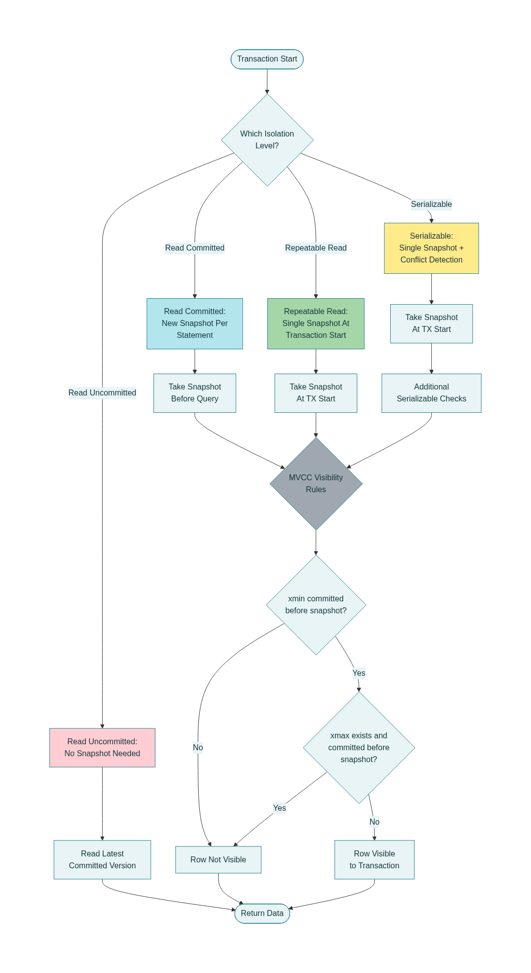
• Serializable: This is the highest isolation level, which in PostgreSQL is an extension of snapshot isolation with additional checks to ensure truly serializable execution. PostgreSQL implements Serializable by using Serializable Snapshot Isolation (SSI). Like Repeatable Read, each transaction gets a single snapshot for its duration. In addition, the system monitors concurrent transactions for patterns that could lead to serialization anomalies (e.g., the classic write skew or other anomalies that snapshot isolation alone doesn’t prevent). If such a pattern is detected, PostgreSQL will roll back one of the involved transactions with a serialization failure error. This forces the application to retry that transaction, and in doing so ensures the outcome is equivalent to some serial (one-at-a-time) order of execution. Serializable isolation in PostgreSQL thus prevents all phenomena (no dirty read, no non-repeatable read, no phantoms, no write-skew anomalies) at the cost of needing to handle occasional transaction aborts. Importantly, PostgreSQL achieves this without heavy locking – it uses a mix of MVCC + locks on predicate (ranges) and a “dangerous structure” detection algorithm to decide when to abort transactions that can’t be safely ordered. From the application perspective, you just get serialization errors if a conflict occurred; if none do, the effect is as if transactions executed in some sequential order.
• Read Uncommitted: PostgreSQL does not actually have a dirty-read isolation level – if you request Read Uncommitted, you get Read Committed behavior. This is because reading uncommitted data (dirty reads) is not possible under PostgreSQL’s MVCC without violating architecture; and it’s rarely useful. So PostgreSQL internally maps “Read Uncommitted” to “Read Committed” for all practical purposes.

In summary, PostgreSQL’s MVCC allows concurrent transactions to proceed with minimal blocking: readers never wait for writers (they see an appropriate snapshot of data), and writers only wait if they conflict on the same row. Row-level locks are still used for modifying data to prevent two transactions from trying to concurrently modify the same row. For example, if Transaction X tries to update a row that Transaction Y is also updating, one will lock the row first; the second will detect the row is already locked (the first update’s xmax) and will wait for Y to commit or abort. If Y commits, X will see that a newer version exists and either retry its update on the new version or abort in case of a conflict (to avoid lost updates). This ensures no lost updates: concurrent updates are serialized on a per-row basis. Reads, however, do not lock out writers – a writer only briefly takes a lock to insert/delete a tuple (and that doesn’t block readers because readers ignore those locks and use versioning).

Vacuum and Wraparound: An important aspect of transaction management is the VACUUM process. Since old, obsolete row versions remain after updates/deletes (for MVCC), PostgreSQL must periodically clean them up to reclaim space – this is what VACUUM does. The autovacuum background workers automatically vacuum tables in the background. Vacuuming not only removes dead tuples but also updates the visibility map (marking pages all-frozen or all-visible when appropriate) and prevents transaction ID wraparound. PostgreSQL’s transaction IDs are 32-bit and will eventually wrap around. To guard against reuse of XIDs that are still in use in some tuple headers, PostgreSQL freezes very old tuples (replacing their xmin with a “frozen” transaction ID that is universally considered committed in the distant past) once their XIDs are old enough. Autovacuum takes care of this freezing as needed. If vacuum is not run, the database can eventually refuse transactions to avoid wraparound issues. Thus, MVCC’s robustness depends on routine vacuuming – which PostgreSQL handles automatically in most cases.

SQL & Data Modeling

PostgreSQL Data Types Hierarchy Chart

Data Types

PostgreSQL provides a rich ecosystem of data types that can be categorized into three main groups: primitive, composite, and special types. Understanding these types is crucial for optimal database design and performance. postgresql.org neon.com

Primitive Data Types

Numeric Types form the backbone of quantitative data storage. PostgreSQL offers various integer types including INTEGER (4 bytes), BIGINT (8 bytes), and SERIAL for auto-incrementing sequences. For precise decimal calculations, NUMERIC(precision, scale) provides exact arithmetic, essential for financial applications where floating-point errors are unacceptable. scribd.com youtube.com

Character Types handle textual data with three main variants: CHAR(n) for fixed-length strings, VARCHAR(n) for variable-length strings with limits, and TEXT for unlimited-length strings. The choice between these impacts storage efficiency and query performance.

Boolean and Temporal Types complete the primitive category. BOOLEAN stores true/false values with PostgreSQL accepting various input formats (1, yes, y, t, true convert to true). Temporal types include DATE, TIME, TIMESTAMP, and INTERVAL for comprehensive time-based data management.

Composite Data Types

Arrays enable storage of multiple values of the same type in a single column. PostgreSQL supports both single and multi-dimensional arrays: integer[], text[], or integer for fixed dimensions. This feature proves invaluable for storing related data without normalization overhead openstax.org

JSON and JSONB Types revolutionize semi-structured data storage. While JSON stores exact input text, JSONB uses binary format for faster processing and supports indexing. JSONB removes insignificant whitespace and reorders keys, making it ideal for applications requiring JSON query performance. tigerdata.com

hstore provides key-value pair storage within a single column, excellent for storing attributes that vary between records. The syntax uses "key"=>"value" pairs separated by commas, and it supports indexing with GIN indexes for efficient queries. geeksforgeeks.org dbvis.com neon.com

Special Data Types

Geospatial Types through PostGIS extension add GEOMETRY and GEOGRAPHY types for location-based applications. These types support points, lines, polygons, and complex spatial operations essential for GIS applications. neon.com tigerdata.com

Network Types including INET, CIDR, and MACADDR provide specialized storage for network-related data, ensuring proper validation and efficient storage.

UUID type stores universally unique identifiers, crucial for distributed systems and ensuring global uniqueness across databases.

SQL example showing primary key in a department table and foreign key in an employee table to illustrate relational constraint

Primary and Foreign Keys

Primary Keys serve as unique row identifiers, combining NOT NULL and UNIQUE constraints. They can be single columns or composite keys spanning multiple columns. PostgreSQL automatically creates a unique B-tree index on primary key columns. prisma.io

Foreign Keys establish referential integrity between tables using the REFERENCES constraint. They support various actions: ON DELETE CASCADE removes child records when parent is deleted, while ON UPDATE RESTRICT prevents parent updates if children exist. Foreign keys can reference primary keys or any unique constraint. tigerdata

Unique and Check Constraints

Unique Constraints ensure no duplicate values while allowing NULL values. They can span multiple columns, ensuring uniqueness of combinations rather than individual values. navicat.com

Check Constraints enforce domain-specific rules using custom conditions. Examples include price > 0 or complex business rules like (category = 'premium' AND price >= 100). They provide flexible validation beyond simple data type checking. neon.com

Advanced Constraint Types

Exclusion Constraints prevent conflicting data using custom operators. They’re particularly useful for preventing overlapping time ranges: EXCLUDE USING GIST (room_id WITH =, daterange(check_in, check_out) WITH &&). This PostgreSQL-specific feature provides powerful conflict resolution.

 1
 2
 3
 4
 5
 6
 7
 8
 9
10
11
12
13
14
15
16
17
18
19
20
21
22
23
24
25
26
27
28
29
30
31
32
33
34
35
36
37
38
39
40
41
42
43
44
45
46
47
48
49
50
51
52
53
54
55
56
57
58
59
60
61
62
63
64
65
66
67
68
69
70
71
72
73
74
75
76
77
78
79
80
81
82
83
84
85
86
87
88
89
90
91

-- CONSTRAINTS AND KEYS EXAMPLES

-- Primary Key Constraints
CREATE TABLE customers (
    customer_id SERIAL PRIMARY KEY,        -- Single column primary key
    email VARCHAR(100) UNIQUE NOT NULL,
    first_name VARCHAR(50) NOT NULL,
    last_name VARCHAR(50) NOT NULL,
    created_at TIMESTAMP DEFAULT NOW()
);

-- Composite Primary Key
CREATE TABLE order_items (
    order_id INTEGER,
    product_id INTEGER,
    quantity INTEGER NOT NULL,
    unit_price NUMERIC(10,2) NOT NULL,
    PRIMARY KEY (order_id, product_id)     -- Composite primary key
);

-- Foreign Key Constraints
CREATE TABLE orders (
    order_id SERIAL PRIMARY KEY,
    customer_id INTEGER NOT NULL,
    order_date DATE DEFAULT CURRENT_DATE,
    total_amount NUMERIC(12,2),

    -- Foreign key with explicit naming and actions
    CONSTRAINT fk_orders_customer 
        FOREIGN KEY (customer_id) 
        REFERENCES customers(customer_id)
        ON DELETE CASCADE                   -- Delete orders when customer is deleted
        ON UPDATE RESTRICT                  -- Prevent customer_id updates if orders exist
);

-- Unique Constraints
CREATE TABLE user_accounts (
    user_id SERIAL PRIMARY KEY,
    username VARCHAR(50) UNIQUE NOT NULL,  -- Column-level unique
    email VARCHAR(100),
    phone VARCHAR(20),

    -- Table-level unique constraint on multiple columns
    CONSTRAINT uk_user_contact UNIQUE (email, phone)
);

-- Check Constraints
CREATE TABLE products (
    product_id SERIAL PRIMARY KEY,
    product_name VARCHAR(100) NOT NULL,
    price NUMERIC(10,2) CHECK (price > 0),              -- Simple check
    discount_percent INTEGER CHECK (discount_percent BETWEEN 0 AND 100),
    category VARCHAR(50),
    stock_quantity INTEGER DEFAULT 0,

    -- Complex check constraint
    CONSTRAINT chk_category_price 
        CHECK (
            (category = 'premium' AND price >= 100) OR 
            (category != 'premium')
        )
);

-- NOT NULL and DEFAULT Constraints
CREATE TABLE employee_records (
    employee_id SERIAL PRIMARY KEY,
    first_name VARCHAR(50) NOT NULL,                    -- Required field
    last_name VARCHAR(50) NOT NULL,
    hire_date DATE DEFAULT CURRENT_DATE,                -- Default to today
    salary NUMERIC(10,2) DEFAULT 50000.00,             -- Default salary
    is_active BOOLEAN DEFAULT true,                     -- Default to active
    department VARCHAR(50) DEFAULT 'General',           -- Default department
    last_updated TIMESTAMP DEFAULT NOW()                -- Auto-timestamp
);

-- Exclusion Constraints (PostgreSQL specific)
CREATE TABLE room_bookings (
    booking_id SERIAL PRIMARY KEY,
    room_id INTEGER NOT NULL,
    guest_name VARCHAR(100) NOT NULL,
    check_in DATE NOT NULL,
    check_out DATE NOT NULL,

    -- Ensure no overlapping bookings for the same room
    CONSTRAINT exclude_overlapping_bookings
        EXCLUDE USING GIST (
            room_id WITH =,
            daterange(check_in, check_out, '[]') WITH &&
        )
);

Indexes: Optimizing Query Performance

PostgreSQL Index Types Comparison Diagram

B-Tree Indexes: The Default Choice

B-Tree indexes handle equality and range queries efficiently, supporting operators <, <=, =, >=, >, BETWEEN, and IN. They maintain sorted data structure, enabling fast lookups and ordered result sets. B-tree indexes work with most data types and support both single and composite column indexing. dev.to neon.com

Hash Indexes: Equality-Only Performance

Hash Indexes excel at exact-match queries using equality operator only. While faster than B-tree for simple equality checks, they cannot handle range queries or provide ordered results. They’re ideal for UUID lookups or exact string matches.

GiST Indexes: Extensible Tree Structures

GiST (Generalized Search Tree) indexes support geometric data types, full-text search, and custom operators. They’re essential for PostGIS spatial queries and can be extended for application-specific data types. GiST indexes enable exclusion constraints and complex geometric operations.

SP-GiST Indexes: Space-Partitioned Trees

SP-GiST (Space-Partitioned GiST) indexes handle non-balanced tree structures efficiently. They excel with point data, ranges, and prefix searches on text data. Unlike balanced trees, SP-GiST adapts to data distribution patterns.

GIN Indexes: Inverted Index Power

GIN (Generalized Inverted Index) indexes optimize queries on composite values like arrays, JSONB, and full-text search. They’re crucial for @> (contains) and && (overlaps) operators on arrays and JSONB queries using @>, ?, and ?& operators. tigerdata

BRIN Indexes: Block Range Efficiency

BRIN (Block Range Index) indexes provide minimal storage overhead for very large tables with naturally ordered data. They store minimum and maximum values per page range, making them ideal for time-series data or sequential identifiers. BRIN indexes can be 100x smaller than equivalent B-tree indexes while maintaining good performance for range queries. enterprisedb.com

Partial and Expression Indexes

Partial Indexes include only rows meeting specific conditions, reducing index size and maintenance overhead. Examples include indexing only active users: CREATE INDEX ON users (email) WHERE active = true. geeksforgeeks neon yugabyte

Expression Indexes enable indexing on computed values like LOWER(email) for case-insensitive searches or EXTRACT(year FROM order_date) for date-based queries. They pre-compute expensive operations, significantly improving query performance.

  1
  2
  3
  4
  5
  6
  7
  8
  9
 10
 11
 12
 13
 14
 15
 16
 17
 18
 19
 20
 21
 22
 23
 24
 25
 26
 27
 28
 29
 30
 31
 32
 33
 34
 35
 36
 37
 38
 39
 40
 41
 42
 43
 44
 45
 46
 47
 48
 49
 50
 51
 52
 53
 54
 55
 56
 57
 58
 59
 60
 61
 62
 63
 64
 65
 66
 67
 68
 69
 70
 71
 72
 73
 74
 75
 76
 77
 78
 79
 80
 81
 82
 83
 84
 85
 86
 87
 88
 89
 90
 91
 92
 93
 94
 95
 96
 97
 98
 99
100
101
102
103
104
105
106
107
108
109
110
111
112
113
114
115
116
117
118
119
120
121
122
123
124
125
126
127
128
129
130
131
132
133
134
135
136
137
138
139
140
141
142
143
144
145
146
147
148
149
150
151
152
153
154
155
156
157
158
159
160
161
162
163
164
165
166
167
168
169
170
171
172
173
174
175
176
177
178
179
180
181
182
183
184
185
186
187
188
189
190
191
192
193
194
195
196
197
198
199
200
201
202
203
204
205
206
207
208
209
210
211
212
213
214

- POSTGRESQL INDEXES DEEP DIVE EXAMPLES

-- B-TREE INDEXES (Default Index Type)
-- Best for: Equality and range queries, sorting operations

-- Simple B-tree index
CREATE INDEX idx_customers_email ON customers (email);

-- Composite B-tree index (multiple columns)
CREATE INDEX idx_orders_customer_date ON orders (customer_id, order_date);

-- Partial B-tree index (with WHERE clause)
CREATE INDEX idx_orders_active ON orders (order_date) 
WHERE status = 'active';

-- Expression index (on computed values)
CREATE INDEX idx_customers_lower_email ON customers (LOWER(email));

-- B-tree index with specific sort order
CREATE INDEX idx_products_price_desc ON products (price DESC, product_name ASC);

-- HASH INDEXES
-- Best for: Simple equality comparisons only (=)

-- Hash index for exact matches
CREATE INDEX idx_users_username_hash ON users USING HASH (username);

-- Hash index on UUID (good for exact lookups)
CREATE INDEX idx_sessions_token_hash ON user_sessions USING HASH (session_id);

-- GiST INDEXES (Generalized Search Tree)
-- Best for: Geometric data, full-text search, range types

-- GiST index for geometric data (requires PostGIS)
CREATE INDEX idx_locations_geom ON locations USING GIST (location);

-- GiST index for range data
CREATE TABLE reservations (
    id SERIAL PRIMARY KEY,
    room_id INTEGER,
    reservation_period DATERANGE
);

CREATE INDEX idx_reservations_period ON reservations USING GIST (reservation_period);

-- GiST index for exclusion constraints
CREATE INDEX idx_bookings_exclusion ON room_bookings 
USING GIST (room_id, daterange(check_in, check_out, '[]'));

-- SP-GiST INDEXES (Space-Partitioned GiST)
-- Best for: Non-balanced tree structures, points, ranges

-- SP-GiST index for point data
CREATE TABLE spatial_points (
    id SERIAL PRIMARY KEY,
    point_data POINT
);

CREATE INDEX idx_points_spgist ON spatial_points USING SPGIST (point_data);

-- SP-GiST index for text (prefix searches)
CREATE INDEX idx_products_name_spgist ON products USING SPGIST (product_name);

-- GIN INDEXES (Generalized Inverted Index)
-- Best for: Arrays, JSONB, full-text search, composite values

-- GIN index for array columns
CREATE INDEX idx_products_tags ON product_catalog USING GIN (tags);

-- GIN index for JSONB data
CREATE INDEX idx_user_metadata ON user_preferences USING GIN (metadata);

-- GIN index for full-text search
CREATE INDEX idx_products_fulltext ON products USING GIN (to_tsvector('english', product_name || ' ' || description));

-- GIN index for hstore
CREATE INDEX idx_product_attributes ON product_attributes USING GIN (attributes);

-- BRIN INDEXES (Block Range Index)
-- Best for: Very large tables with naturally ordered data

-- BRIN index for timestamp columns (time-series data)
CREATE TABLE sensor_readings (
    id BIGSERIAL PRIMARY KEY,
    sensor_id INTEGER,
    reading_value NUMERIC(10,2),
    recorded_at TIMESTAMP DEFAULT NOW()
);

CREATE INDEX idx_readings_time_brin ON sensor_readings USING BRIN (recorded_at);

-- BRIN index for sequential data
CREATE INDEX idx_readings_id_brin ON sensor_readings USING BRIN (id);

-- PARTIAL INDEXES Examples
-- Include only subset of rows based on conditions

-- Index only active users
CREATE INDEX idx_users_active_email ON users (email) 
WHERE is_active = true;

-- Index only recent orders (last 30 days)
CREATE INDEX idx_recent_orders ON orders (order_date, customer_id) 
WHERE order_date >= (CURRENT_DATE - INTERVAL '30 days');

-- Index only high-value orders
CREATE INDEX idx_high_value_orders ON orders (customer_id, total_amount) 
WHERE total_amount > 1000;

-- Index only non-null values
CREATE INDEX idx_customers_phone ON customers (phone) 
WHERE phone IS NOT NULL;

-- EXPRESSION INDEXES Examples
-- Index on computed or transformed values

-- Case-insensitive search
CREATE INDEX idx_customers_email_lower ON customers (LOWER(email));

-- Date parts
CREATE INDEX idx_orders_year_month ON orders (EXTRACT(year FROM order_date), EXTRACT(month FROM order_date));

-- String functions
CREATE INDEX idx_products_name_length ON products (LENGTH(product_name));

-- Mathematical expressions
CREATE INDEX idx_products_profit_margin ON products ((price - cost) / cost * 100);

-- UNIQUE INDEXES
-- Enforce uniqueness while providing index benefits

-- Unique index on single column
CREATE UNIQUE INDEX idx_users_email_unique ON users (email);

-- Unique index on multiple columns
CREATE UNIQUE INDEX idx_user_social_unique ON users (provider, social_id) 
WHERE provider IS NOT NULL AND social_id IS NOT NULL;

-- Conditional unique index
CREATE UNIQUE INDEX idx_users_username_active ON users (username) 
WHERE is_active = true;

-- COVERING INDEXES (INCLUDE clause)
-- Include additional columns in index for index-only scans

-- B-tree index with included columns
CREATE INDEX idx_orders_customer_include ON orders (customer_id) 
INCLUDE (order_date, total_amount, status);

-- CONCURRENT INDEX CREATION
-- Create indexes without blocking writes (for production)

-- Create index concurrently (non-blocking)
CREATE INDEX CONCURRENTLY idx_products_category ON products (category);

-- Drop index concurrently
DROP INDEX CONCURRENTLY idx_old_products_name;

-- INDEX MAINTENANCE EXAMPLES

-- Check index usage statistics
SELECT 
    schemaname,
    tablename,
    indexname,
    idx_scan,
    idx_tup_read,
    idx_tup_fetch
FROM pg_stat_user_indexes 
ORDER BY idx_scan DESC;

-- Check index sizes
SELECT 
    indexname,
    pg_size_pretty(pg_relation_size(indexname::regclass)) as size
FROM pg_indexes 
WHERE schemaname = 'public'
ORDER BY pg_relation_size(indexname::regclass) DESC;

-- Reindex for maintenance
REINDEX INDEX idx_customers_email;
REINDEX TABLE customers;

-- Example queries that benefit from different index types:

-- B-tree index usage
EXPLAIN (ANALYZE, BUFFERS) 
SELECT * FROM customers 
WHERE email = 'john@example.com';

-- Range query with B-tree
EXPLAIN (ANALYZE, BUFFERS) 
SELECT * FROM orders 
WHERE order_date BETWEEN '2025-01-01' AND '2025-12-31';

-- Hash index usage
EXPLAIN (ANALYZE, BUFFERS) 
SELECT * FROM users 
WHERE username = 'johndoe123';

-- GIN index for array queries
EXPLAIN (ANALYZE, BUFFERS) 
SELECT * FROM product_catalog 
WHERE tags @> ARRAY['electronics'];

-- GIN index for JSONB queries
EXPLAIN (ANALYZE, BUFFERS) 
SELECT * FROM user_preferences 
WHERE metadata @> '{"last_login": "2025-10-02"}';

-- BRIN index for range queries on large tables
EXPLAIN (ANALYZE, BUFFERS) 
SELECT * FROM sensor_readings 
WHERE recorded_at >= '2025-10-01';

Advanced SQL Features: Leveraging PostgreSQL’s Power

SQL Window Functions Diagram

Window Functions: Analytical Processing

Window Functions perform calculations across row sets related to the current row without grouping results. They include:

• Ranking Functions like ROW_NUMBER(), RANK(), DENSE_RANK() assign positions within ordered sets. PERCENT_RANK() calculates percentage rankings for statistical analysis. tigerdata datalemur
• Lag and Lead Functions access previous or subsequent rows using LAG() and LEAD(). These functions enable time-series analysis, calculating period-over-period changes without self-joins: LAG(sales) OVER (PARTITION BY product ORDER BY date). codedamn neon
• Aggregate Window Functions like SUM() OVER(), AVG() OVER() provide running totals and moving averages. Frame clauses control calculation windows: ROWS BETWEEN UNBOUNDED PRECEDING AND CURRENT ROW.

Common Table Expressions (CTEs): Query Organization

CTEs create named temporary result sets improving query readability and reusability. They support multiple CTEs in single queries and can reference each other sequentially. CTEs excel at breaking complex queries into manageable components. neon

Recursive CTEs handle hierarchical data using WITH RECURSIVE syntax. They consist of anchor members (base case) and recursive members (iterative case), perfect for organizational charts, bill-of-materials, or graph traversal. cybertec-postgresql geeksforgeeks

Upserts and ON CONFLICT: Data Synchronization

INSERT ON CONFLICT provides atomic upsert operations combining insert and update logic. Two main actions handle conflicts:

• DO NOTHING silently ignores conflicts, useful for “insert if not exists” scenarios
• DO UPDATE modifies existing rows using EXCLUDED pseudo-table to access proposed values. Conditional updates enable sophisticated conflict resolution: DO UPDATE SET price = LEAST(table.price, EXCLUDED.price). geshan
• EXCLUDED Table provides access to values that would have been inserted, enabling complex upsert logic. This virtual table supports all proposed column values and can be used in WHERE clauses for conditional updates.

  1
  2
  3
  4
  5
  6
  7
  8
  9
 10
 11
 12
 13
 14
 15
 16
 17
 18
 19
 20
 21
 22
 23
 24
 25
 26
 27
 28
 29
 30
 31
 32
 33
 34
 35
 36
 37
 38
 39
 40
 41
 42
 43
 44
 45
 46
 47
 48
 49
 50
 51
 52
 53
 54
 55
 56
 57
 58
 59
 60
 61
 62
 63
 64
 65
 66
 67
 68
 69
 70
 71
 72
 73
 74
 75
 76
 77
 78
 79
 80
 81
 82
 83
 84
 85
 86
 87
 88
 89
 90
 91
 92
 93
 94
 95
 96
 97
 98
 99
100
101
102
103
104
105
106
107
108
109
110
111
112
113
114
115
116
117
118
119
120
121
122
123
124
125
126
127
128
129
130
131
132
133
134
135
136
137
138
139
140
141
142
143
144
145
146
147
148
149
150
151
152
153
154
155
156
157
158
159
160
161
162
163
164
165
166
167
168
169
170
171
172
173
174
175
176
177
178
179
180
181
182
183
184
185
186
187
188
189
190
191
192
193
194
195
196
197
198
199
200
201
202
203
204
205
206
207
208
209
210
211
212
213
214
215
216
217
218
219
220
221
222
223
224
225
226
227
228
229
230
231
232
233
234
235
236
237
238
239
240
241
242
243
244
245
246
247
248
249
250
251
252
253
254
255
256
257
258
259
260
261
262
263
264
265
266
267
268
269
270
271
272
273
274
275
276
277
278
279
280
281
282
283
284
285
286
287
288
289
290
291
292
293
294
295
296
297
298
299
300
301
302
303
304
305
306
307
308
309
310
311
312
313
314
315
316
317
318
319
320
321
322
323
324
325
326
327
328
329
330
331
332
333
334
335
336
337
338
339
340
341
342
343
344
345
346
347
348
349
350
351
352
353
354
355
356
357
358
359
360
361
362
363
364
365
366
367

- ADVANCED SQL FEATURES IN POSTGRESQL

-- WINDOW FUNCTIONS Examples
-- Perform calculations across sets of rows related to current row

-- Sample data setup
CREATE TABLE sales_performance (
    id SERIAL PRIMARY KEY,
    salesperson VARCHAR(50),
    region VARCHAR(50),
    quarter INTEGER,
    year INTEGER,
    sales_amount NUMERIC(12,2),
    sale_date DATE
);

INSERT INTO sales_performance (salesperson, region, quarter, year, sales_amount, sale_date) 
VALUES 
    ('Alice', 'North', 1, 2025, 50000, '2025-03-15'),
    ('Alice', 'North', 2, 2025, 55000, '2025-06-15'),
    ('Bob', 'South', 1, 2025, 48000, '2025-03-10'),
    ('Bob', 'South', 2, 2025, 52000, '2025-06-10'),
    ('Carol', 'North', 1, 2025, 51000, '2025-03-20'),
    ('Carol', 'North', 2, 2025, 49000, '2025-06-20');

-- ROW_NUMBER() - Assigns unique sequential integers
SELECT 
    salesperson,
    region,
    sales_amount,
    ROW_NUMBER() OVER (ORDER BY sales_amount DESC) as overall_rank,
    ROW_NUMBER() OVER (PARTITION BY region ORDER BY sales_amount DESC) as region_rank
FROM sales_performance;

-- RANK() and DENSE_RANK() - Handle ties differently
SELECT 
    salesperson,
    sales_amount,
    RANK() OVER (ORDER BY sales_amount DESC) as rank_with_gaps,
    DENSE_RANK() OVER (ORDER BY sales_amount DESC) as dense_rank,
    PERCENT_RANK() OVER (ORDER BY sales_amount DESC) as percent_rank
FROM sales_performance;

-- LAG() and LEAD() - Access previous/next rows
SELECT 
    salesperson,
    quarter,
    sales_amount,
    LAG(sales_amount) OVER (PARTITION BY salesperson ORDER BY quarter) as previous_quarter,
    LEAD(sales_amount) OVER (PARTITION BY salesperson ORDER BY quarter) as next_quarter,
    sales_amount - LAG(sales_amount) OVER (PARTITION BY salesperson ORDER BY quarter) as growth
FROM sales_performance;

-- FIRST_VALUE() and LAST_VALUE() - Get first/last values in window
SELECT 
    salesperson,
    quarter,
    sales_amount,
    FIRST_VALUE(sales_amount) OVER (
        PARTITION BY salesperson 
        ORDER BY quarter 
        ROWS BETWEEN UNBOUNDED PRECEDING AND UNBOUNDED FOLLOWING
    ) as first_quarter_sales,
    LAST_VALUE(sales_amount) OVER (
        PARTITION BY salesperson 
        ORDER BY quarter 
        ROWS BETWEEN UNBOUNDED PRECEDING AND UNBOUNDED FOLLOWING
    ) as last_quarter_sales
FROM sales_performance;

-- NTILE() - Divide rows into groups
SELECT 
    salesperson,
    sales_amount,
    NTILE(3) OVER (ORDER BY sales_amount DESC) as performance_tier
FROM sales_performance;

-- Cumulative calculations with window functions
SELECT 
    salesperson,
    quarter,
    sales_amount,
    SUM(sales_amount) OVER (PARTITION BY salesperson ORDER BY quarter) as cumulative_sales,
    AVG(sales_amount) OVER (PARTITION BY salesperson ORDER BY quarter) as running_average,
    COUNT(*) OVER (PARTITION BY salesperson ORDER BY quarter) as quarters_completed
FROM sales_performance;

-- COMMON TABLE EXPRESSIONS (CTEs)
-- Named temporary result sets for complex queries

-- Simple CTE
WITH high_performers AS (
    SELECT 
        salesperson,
        region,
        AVG(sales_amount) as avg_sales
    FROM sales_performance
    GROUP BY salesperson, region
    HAVING AVG(sales_amount) > 50000
)
SELECT 
    hp.salesperson,
    hp.region,
    hp.avg_sales,
    sp.sales_amount,
    sp.quarter
FROM high_performers hp
JOIN sales_performance sp ON hp.salesperson = sp.salesperson;

-- Multiple CTEs
WITH quarterly_totals AS (
    SELECT 
        quarter,
        SUM(sales_amount) as total_sales,
        COUNT(*) as num_sales
    FROM sales_performance
    GROUP BY quarter
),
regional_totals AS (
    SELECT 
        region,
        SUM(sales_amount) as total_sales,
        AVG(sales_amount) as avg_sales
    FROM sales_performance
    GROUP BY region
)
SELECT 
    'Q' || qt.quarter as period,
    qt.total_sales as quarter_total,
    rt.region,
    rt.total_sales as region_total
FROM quarterly_totals qt
CROSS JOIN regional_totals rt;

-- RECURSIVE QUERIES
-- Handle hierarchical data structures

-- Sample hierarchical data
CREATE TABLE employees (
    employee_id SERIAL PRIMARY KEY,
    name VARCHAR(100),
    manager_id INTEGER REFERENCES employees(employee_id),
    department VARCHAR(50),
    salary NUMERIC(10,2)
);

INSERT INTO employees (name, manager_id, department, salary) VALUES
    ('CEO John', NULL, 'Executive', 200000),
    ('VP Alice', 1, 'Sales', 150000),
    ('VP Bob', 1, 'Engineering', 160000),
    ('Manager Carol', 2, 'Sales', 100000),
    ('Manager Dave', 3, 'Engineering', 110000),
    ('Rep Emma', 4, 'Sales', 60000),
    ('Rep Frank', 4, 'Sales', 65000),
    ('Dev Grace', 5, 'Engineering', 85000),
    ('Dev Henry', 5, 'Engineering', 90000);

-- Recursive CTE to find all subordinates
WITH RECURSIVE employee_hierarchy AS (
    -- Anchor member: start with a specific manager
    SELECT 
        employee_id,
        name,
        manager_id,
        department,
        salary,
        0 as level,
        name as path
    FROM employees
    WHERE manager_id IS NULL  -- Start with CEO

    UNION ALL

    -- Recursive member: find direct reports
    SELECT 
        e.employee_id,
        e.name,
        e.manager_id,
        e.department,
        e.salary,
        eh.level + 1,
        eh.path || ' -> ' || e.name
    FROM employees e
    INNER JOIN employee_hierarchy eh ON e.manager_id = eh.employee_id
)
SELECT 
    employee_id,
    REPEAT('  ', level) || name as hierarchical_name,
    level,
    department,
    salary,
    path
FROM employee_hierarchy
ORDER BY level, name;

-- Calculate subordinate counts recursively
WITH RECURSIVE subordinate_counts AS (
    -- Leaf nodes (employees with no direct reports)
    SELECT 
        employee_id,
        name,
        0 as direct_reports,
        0 as total_subordinates
    FROM employees e1
    WHERE NOT EXISTS (
        SELECT 1 FROM employees e2 WHERE e2.manager_id = e1.employee_id
    )

    UNION ALL

    -- Managers with their subordinate counts
    SELECT 
        m.employee_id,
        m.name,
        COUNT(DISTINCT s.employee_id) as direct_reports,
        COUNT(DISTINCT s.employee_id) + COALESCE(SUM(sc.total_subordinates), 0) as total_subordinates
    FROM employees m
    INNER JOIN employees s ON s.manager_id = m.employee_id
    LEFT JOIN subordinate_counts sc ON sc.employee_id = s.employee_id
    GROUP BY m.employee_id, m.name
)
SELECT * FROM subordinate_counts
ORDER BY total_subordinates DESC;

-- UPSERTS and ON CONFLICT
-- Handle insert conflicts gracefully

-- Sample table for upsert examples
CREATE TABLE inventory (
    product_id INTEGER PRIMARY KEY,
    product_name VARCHAR(100),
    quantity INTEGER,
    price NUMERIC(10,2),
    last_updated TIMESTAMP DEFAULT NOW()
);

-- Simple upsert with DO NOTHING
INSERT INTO inventory (product_id, product_name, quantity, price) 
VALUES (1, 'Laptop', 10, 999.99)
ON CONFLICT (product_id) DO NOTHING;

-- Upsert with UPDATE on conflict
INSERT INTO inventory (product_id, product_name, quantity, price) 
VALUES (1, 'Gaming Laptop', 15, 1299.99)
ON CONFLICT (product_id) 
DO UPDATE SET 
    product_name = EXCLUDED.product_name,
    quantity = EXCLUDED.quantity,
    price = EXCLUDED.price,
    last_updated = NOW();

-- Conditional upsert (only update if new price is lower)
INSERT INTO inventory (product_id, product_name, quantity, price) 
VALUES (1, 'Budget Laptop', 20, 799.99)
ON CONFLICT (product_id) 
DO UPDATE SET 
    product_name = EXCLUDED.product_name,
    quantity = inventory.quantity + EXCLUDED.quantity,
    price = LEAST(inventory.price, EXCLUDED.price),
    last_updated = NOW()
WHERE EXCLUDED.price < inventory.price;

-- Upsert with composite unique constraint
CREATE TABLE user_sessions_v2 (
    user_id INTEGER,
    session_date DATE,
    session_count INTEGER DEFAULT 1,
    last_activity TIMESTAMP DEFAULT NOW(),
    PRIMARY KEY (user_id, session_date)
);

INSERT INTO user_sessions_v2 (user_id, session_date, session_count) 
VALUES (123, CURRENT_DATE, 1)
ON CONFLICT (user_id, session_date) 
DO UPDATE SET 
    session_count = user_sessions_v2.session_count + 1,
    last_activity = NOW();

-- ADVANCED CTE with Window Functions
WITH monthly_sales AS (
    SELECT 
        salesperson,
        EXTRACT(month FROM sale_date) as month,
        SUM(sales_amount) as monthly_total
    FROM sales_performance
    GROUP BY salesperson, EXTRACT(month FROM sale_date)
),
sales_with_metrics AS (
    SELECT 
        salesperson,
        month,
        monthly_total,
        AVG(monthly_total) OVER (PARTITION BY salesperson) as personal_avg,
        LAG(monthly_total) OVER (PARTITION BY salesperson ORDER BY month) as prev_month,
        RANK() OVER (PARTITION BY salesperson ORDER BY monthly_total DESC) as month_rank
    FROM monthly_sales
)
SELECT 
    salesperson,
    month,
    monthly_total,
    ROUND(personal_avg, 2) as avg_monthly,
    COALESCE(monthly_total - prev_month, 0) as month_over_month_change,
    CASE 
        WHEN month_rank = 1 THEN 'Best Month'
        WHEN month_rank = (SELECT COUNT(*) FROM monthly_sales ms WHERE ms.salesperson = sales_with_metrics.salesperson) THEN 'Worst Month'
        ELSE 'Regular Month'
    END as performance_label
FROM sales_with_metrics
ORDER BY salesperson, month;

-- Complex query combining multiple advanced features
WITH RECURSIVE territory_hierarchy AS (
    -- Base case: top-level regions
    SELECT 
        region as territory,
        region as parent_territory,
        0 as level
    FROM sales_performance
    WHERE region IS NOT NULL
    GROUP BY region

    UNION ALL

    -- Recursive case: could be expanded for sub-regions
    SELECT 
        sp.region,
        th.territory,
        th.level + 1
    FROM sales_performance sp
    JOIN territory_hierarchy th ON sp.region = th.territory
    WHERE th.level < 2  -- Prevent infinite recursion
),
performance_analysis AS (
    SELECT 
        salesperson,
        region,
        sales_amount,
        quarter,
        -- Window functions for analysis
        RANK() OVER (ORDER BY sales_amount DESC) as overall_rank,
        PERCENT_RANK() OVER (PARTITION BY region ORDER BY sales_amount DESC) as region_percentile,
        NTILE(4) OVER (ORDER BY sales_amount DESC) as quartile,
        LAG(sales_amount) OVER (PARTITION BY salesperson ORDER BY quarter) as prev_quarter_sales,
        -- Running totals and averages
        SUM(sales_amount) OVER (PARTITION BY salesperson ORDER BY quarter) as ytd_sales,
        AVG(sales_amount) OVER (PARTITION BY region) as region_avg
    FROM sales_performance
)
SELECT 
    pa.salesperson,
    pa.region,
    pa.sales_amount,
    pa.quarter,
    pa.overall_rank,
    ROUND(pa.region_percentile * 100, 1) || '%' as region_percentile_text,
    pa.quartile,
    COALESCE(pa.sales_amount - pa.prev_quarter_sales, 0) as qoq_growth,
    pa.ytd_sales,
    ROUND(pa.region_avg, 2) as region_average,
    CASE 
        WHEN pa.sales_amount > pa.region_avg * 1.2 THEN 'Exceeds Expectations'
        WHEN pa.sales_amount > pa.region_avg THEN 'Meets Expectations'
        ELSE 'Below Expectations'
    END as performance_rating
FROM performance_analysis pa
ORDER BY pa.overall_rank;

Advanced Query Patterns

Combining CTEs with Window Functions creates powerful analytical queries. Recursive CTEs can calculate hierarchical aggregates while window functions provide ranking and running totals within each level.

Multi-level Recursion handles complex hierarchical structures with level tracking and path construction. Termination conditions prevent infinite recursion, while path concatenation maintains audit trails.

Complex Upsert Logic supports business rules through conditional updates, multi-column conflicts, and aggregate operations during conflict resolution.

Use Cases and Best Practices

Data Type Selection impacts both storage efficiency and query performance. Use INTEGER for typical numeric IDs, BIGINT for high-volume sequences, NUMERIC for financial calculations, and TEXT for variable-length strings. Choose JSONB over JSON for queryable semi-structured data.

Index Strategy requires understanding query patterns. B-tree indexes suit most scenarios, while GIN indexes optimize array and JSONB queries. Partial indexes reduce maintenance overhead for filtered queries, and BRIN indexes handle time-series data efficiently.

Constraint Design enforces business rules at the database level. Foreign keys maintain referential integrity, check constraints validate business logic, and exclusion constraints prevent complex conflicts like time overlaps.

Advanced SQL Optimization leverages window functions for analytical queries, CTEs for complex logic decomposition, and upserts for efficient data synchronization. Recursive queries handle hierarchical data without application-level loops.